```
#### 重要信息
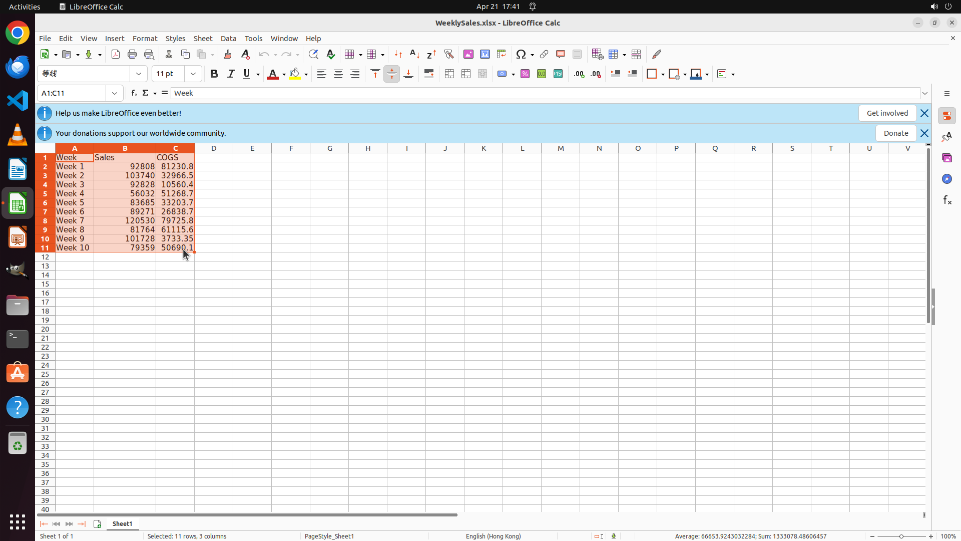
LibreOffice Calc is open with WeeklySales.xlsx file. The spreadsheet contains:
- Column A: Week (Week 1 through Week 10)
- Column B: Sales (values like 92808, 103740, etc.)
- Column C: COGS (values like 81230.8, 32966.5, etc.)
- Data range is A1:C11 (including headers)
- Currently on Sheet1 tab
#### 情况分析与思考过程
I need to complete the task of creating a clustered column chart showing Sales and COGS data for each week in a new sheet named "Sheet2" with the title "Sales & COGS".
According to the strategy tree, the steps are:
1. Select source data range A1:C11 in Sheet1
2. Insert and configure clustered column chart
3. Create destination worksheet "Sheet2"
4. Move chart to Sheet2
The first step is to select the data range A1:C11. I need to click on cell A1 (which contains "Week") and drag to cell C11 (which contains the COGS value for Week 10: 50690.1).
Looking at the screenshot, I can see:
- Cell A1 with "Week" is at the top-left of the data area
- Cell C11 with "50690.1" is in row 11, column C
I'll start by clicking on A1 and dragging to C11 to select the entire data range including headers.
```
Step 1: DRAG_TO (361, 492)
```
#### 重要信息
LibreOffice Calc is open with WeeklySales.xlsx file. The spreadsheet contains:
- Column A: Week (Week 1 through Week 10)
- Column B: Sales (values like 92808, 103740, etc.)
- Column C: COGS (values like 81230.8, 32966.5, etc.)
- Data range is A1:C11 (including headers)
- Currently on Sheet1 tab
#### 情况分析与思考过程
I need to complete the task of creating a clustered column chart showing Sales and COGS data for each week in a new sheet named "Sheet2" with the title "Sales & COGS".
According to the strategy tree, the steps are:
1. Select source data range A1:C11 in Sheet1
2. Insert and configure clustered column chart
3. Create destination worksheet "Sheet2"
4. Move chart to Sheet2
The first step is to select the data range A1:C11. I need to click on cell A1 (which contains "Week") and drag to cell C11 (which contains the COGS value for Week 10: 50690.1).
Looking at the screenshot, I can see:
- Cell A1 with "Week" is at the top-left of the data area
- Cell C11 with "50690.1" is in row 11, column C
I'll start by clicking on A1 and dragging to C11 to select the entire data range including headers.
```
Step 2: CLICK (228, 75)
```
#### 重要信息
The data range A1:C11 has been successfully selected. I can see:
- The range A1:C11 is highlighted (blue/orange selection)
- The cell reference box shows "A1:C11"
- The status bar shows "Selected: 11 rows, 3 columns"
- The data includes Week, Sales, and COGS columns with headers and all 10 weeks of data
#### 情况分析与思考过程
Step 1 of the strategy tree is complete - I've selected the source data range A1:C11. Now I need to proceed with Step 2: Insert and configure the clustered column chart.
The next logical step is to open the Insert menu to access the Chart option. I can see the Insert menu in the menu bar at the top of the screen. I'll click on it to open the dropdown menu, which should contain the Chart option.
After clicking Insert, I expect to see a dropdown menu with various options including Chart, which I'll need to select next.
```
Step 3: CLICK (253, 120)
```
#### 重要信息
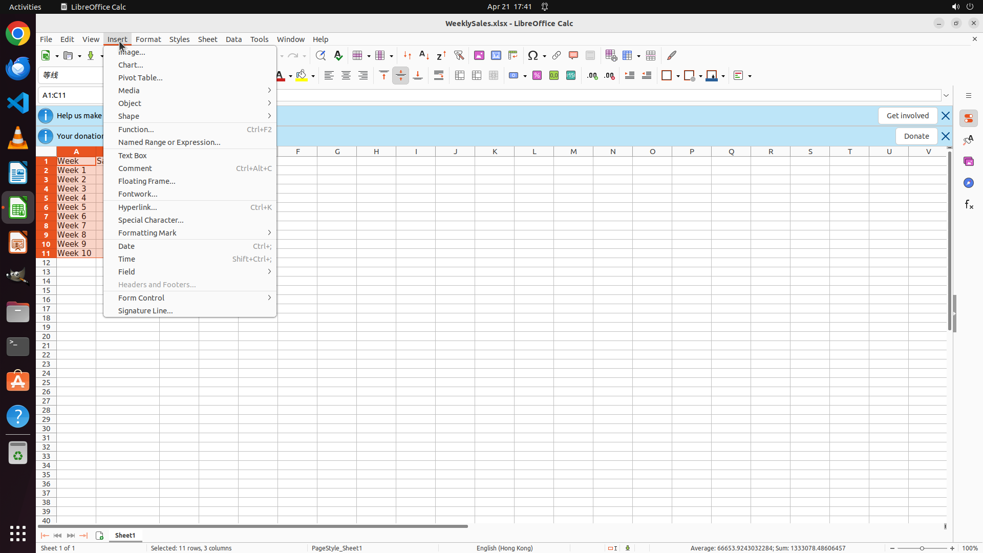
The Insert menu has been successfully opened. I can see:
- The Insert dropdown menu is displayed
- "Chart..." option is visible in the menu
- The data range A1:C11 is still selected (status bar shows "Selected: 11 rows, 3 columns")
#### 情况分析与思考过程
Step 1 (Select source data range) is complete. I've successfully opened the Insert menu as part of Step 2.1. Now I need to click on "Chart..." option to open the chart creation dialog.
After clicking "Chart...", I expect to see a chart wizard or dialog where I can:
1. Select Column chart type
2. Choose Clustered Column subtype
3. Set the chart title to "Sales & COGS"
The logical next action is to click on the "Chart..." option in the Insert menu.
```
Step 4: CLICK (1229, 760)
```
#### 重要信息
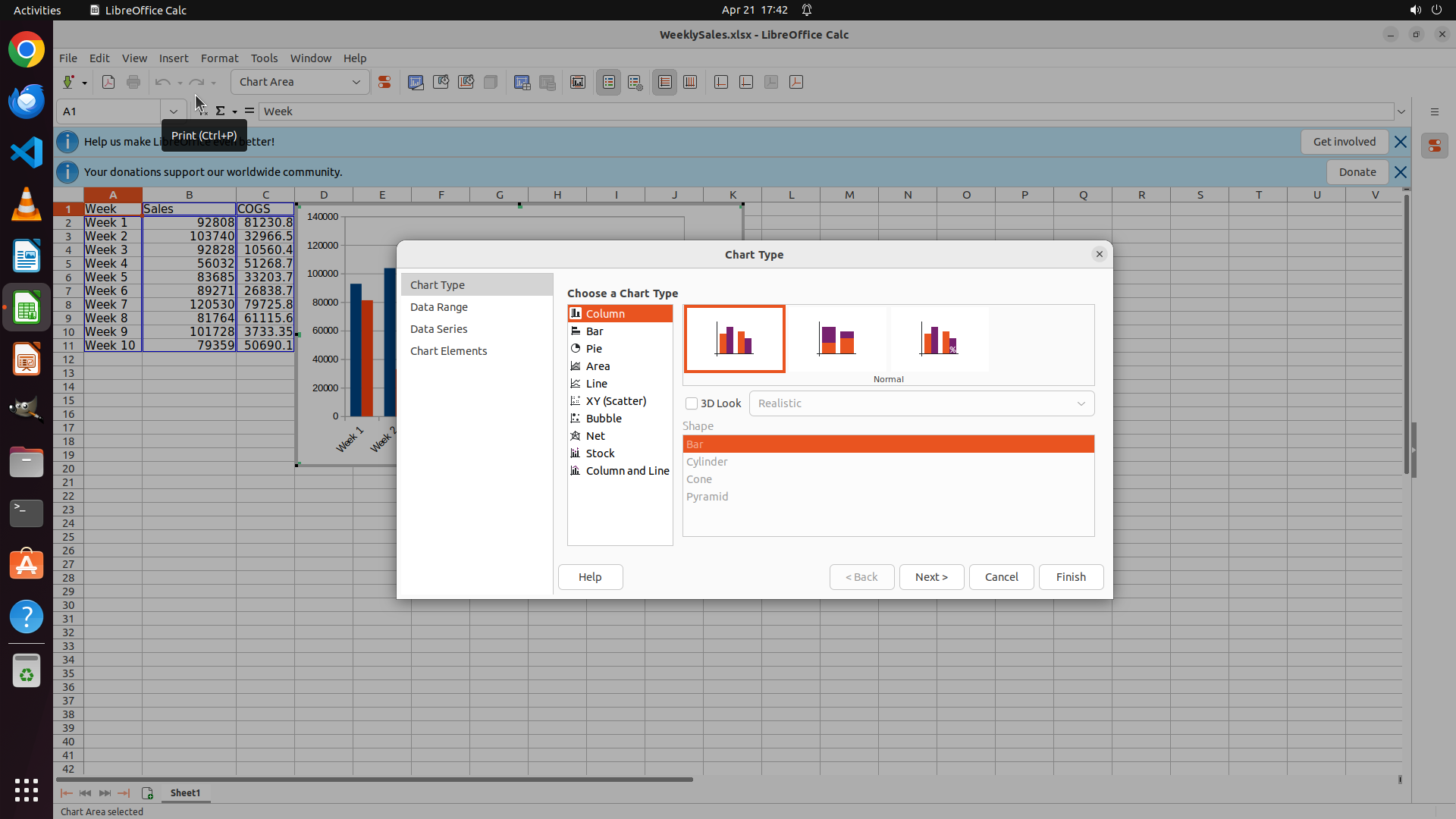
The Chart Type dialog has opened successfully. I can see:
- "Column" chart type is already selected (highlighted in orange on the left)
- The first subtype (clustered column) is already selected with an orange border on the right
- There are navigation buttons at the bottom: Help, < Back, Next >, Cancel, Finish
- The dialog shows a preview of the chart on the left side showing the data
#### 情况分析与思考过程
Step 2.1 is complete - the Chart dialog is open. Step 2.2 is also effectively complete since:
- Column chart type is already selected
- The clustered column subtype (first option) is already selected
Now I need to proceed to the next step where I can set the chart title to "Sales & COGS". I should click "Next >" to continue to the next step of the chart wizard where I can configure chart elements including the title.
After clicking "Next >", I expect to see the next step of the chart wizard, likely "Chart Elements" or a similar step where I can add and configure the chart title.
```
Step 5: CLICK (1229, 762)
```
#### 重要信息
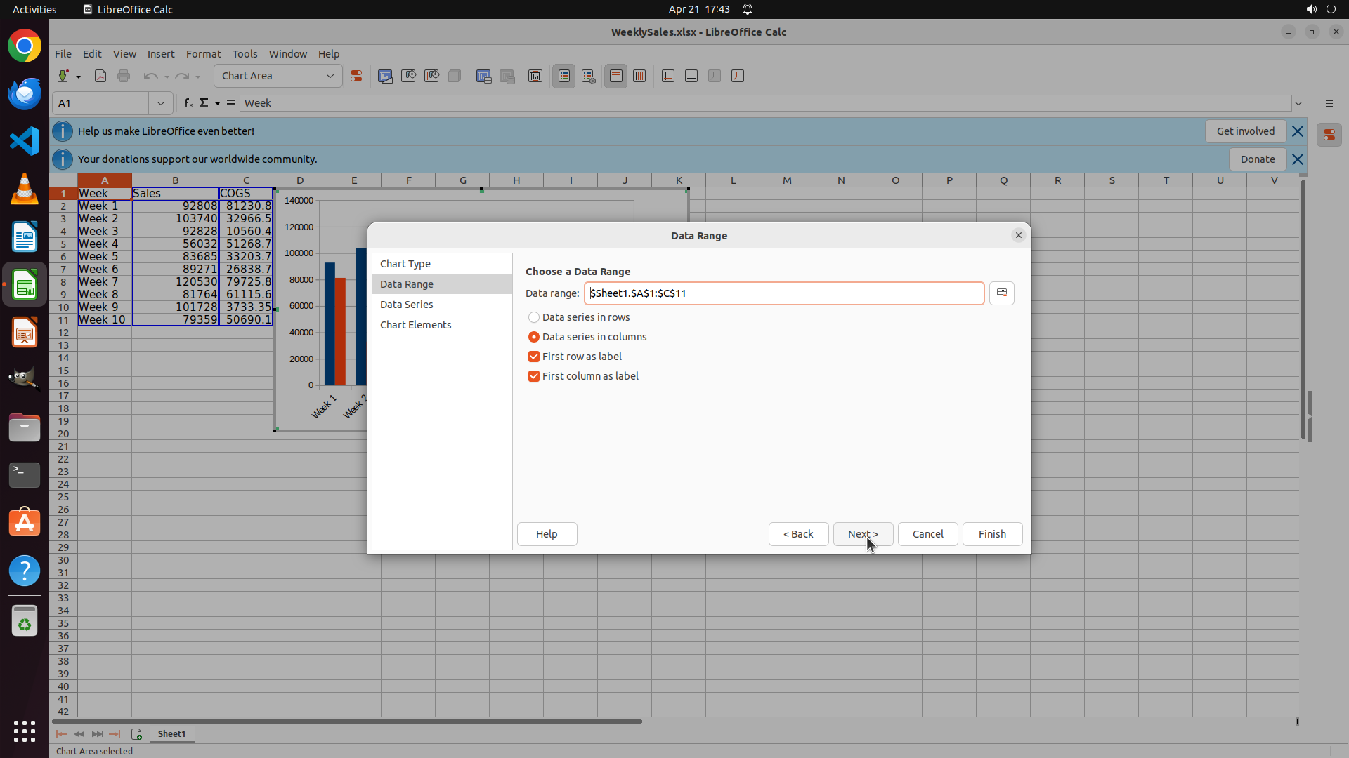
The chart wizard has progressed to the "Data Range" step. I can see:
- Data range is correctly set to "$Sheet1.$A$1:$C$11"
- "Data series in columns" is selected (appropriate since Sales and COGS are separate columns)
- "First row as label" is checked (headers: Week, Sales, COGS)
- "First column as label" is checked (Week 1-10 labels)
- The left sidebar shows the wizard steps: Chart Type, Data Range, Data Series, Chart Elements
- Navigation buttons at bottom: Help, < Back, Next >, Cancel, Finish
#### 情况分析与思考过程
The Data Range step is properly configured with all the correct settings. The data range includes all the necessary data (Week, Sales, COGS for all 10 weeks), and the label options are correctly set.
According to the strategy tree, I need to:
1. ✓ Select data range (completed)
2. ✓ Open Insert > Chart (completed)
3. ✓ Select Column chart type and Clustered Column subtype (completed)
4. → Set chart title to "Sales & COGS" (next step)
5. Create Sheet2 and move chart there (pending)
To set the chart title, I need to proceed to the "Chart Elements" step. I can see in the left sidebar that "Chart Elements" is the last step. I should click "Next >" to continue through the wizard. I may need to go through "Data Series" step first, or I might be able to skip directly to Chart Elements.
The logical next action is to click "Next >" to proceed to the next step of the chart wizard where I can configure the chart title.
```
Step 6: CLICK (1229, 762)
```
#### 重要信息
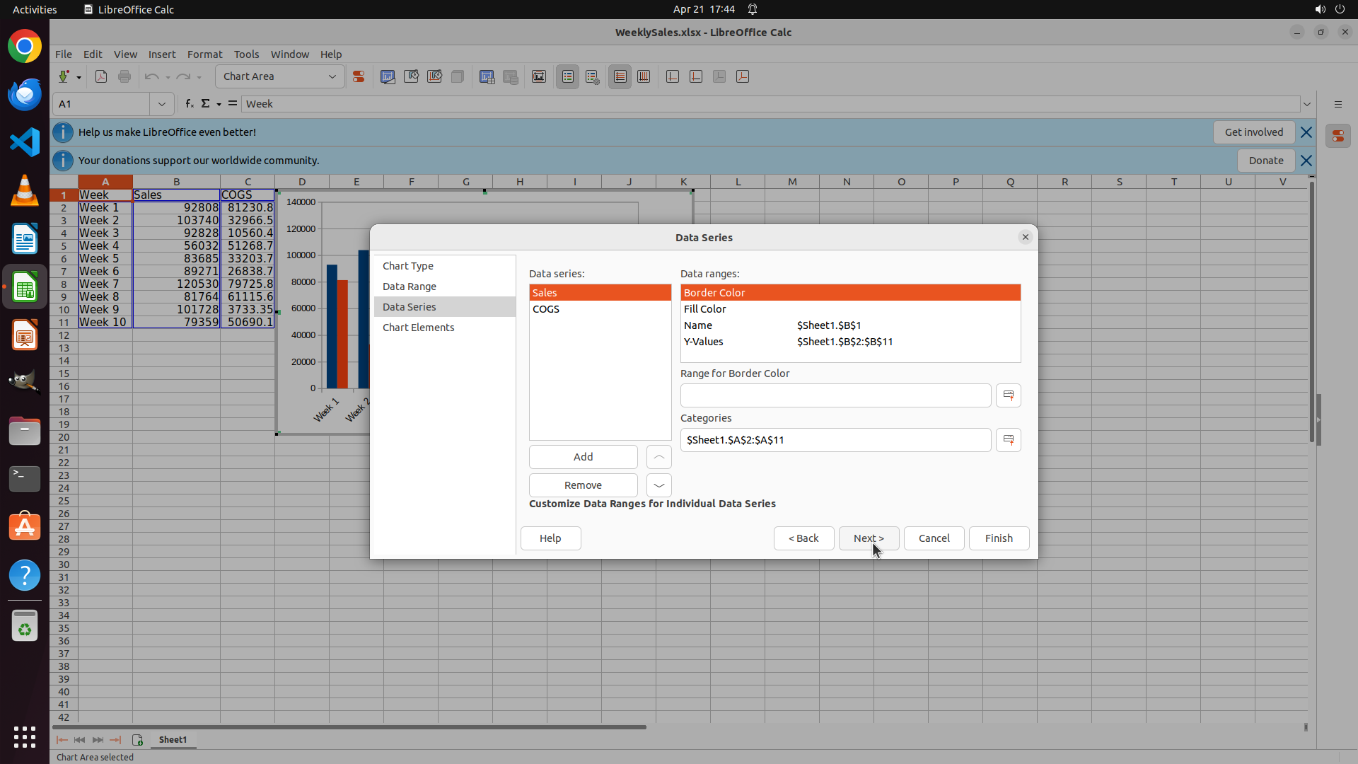
The chart wizard has progressed to the "Data Series" step. I can see:
- Two data series are listed: "Sales" and "COGS"
- Sales series shows Name: $Sheet1.$B$1 and Y-Values: $Sheet1.$B$2:$B$11
- Categories are set to $Sheet1.$A$2:$A$11 (Week 1-10 labels)
- The left sidebar shows the wizard steps: Chart Type, Data Range, Data Series, Chart Elements
- Navigation buttons at bottom: Help, < Back, Next >, Cancel, Finish
#### 情况分析与思考过程
The Data Series step is properly configured with Sales and COGS as separate data series, and Week values as categories. This is exactly what we need for a clustered column chart showing Sales and COGS by Week.
According to the strategy tree, I need to:
1. ✓ Select data range (completed)
2. ✓ Open Insert > Chart (completed)
3. ✓ Select Column chart type and Clustered Column subtype (completed)
4. → Set chart title to "Sales & COGS" (next step)
5. Create Sheet2 and move chart there (pending)
To set the chart title, I need to proceed to the "Chart Elements" step. I can see in the left sidebar that "Chart Elements" is the last step. I should click "Next >" to continue to that step where I can configure the chart title.
The logical next action is to click "Next >" to proceed to the Chart Elements step where I can set the chart title.
```
Step 7: CLICK (1062, 415)
```
#### 重要信息
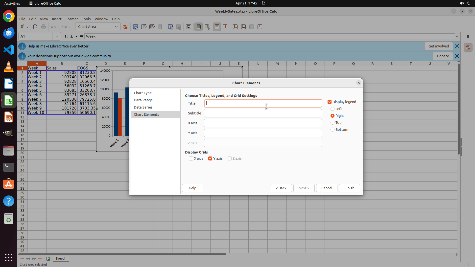
The chart wizard has successfully progressed to the "Chart Elements" step. I can see:
- The "Chart Elements" section is now active (highlighted in the left sidebar)
- There's a "Title" field that's currently empty and ready for input
- The "Display legend" checkbox is checked with "Right" position selected
- The chart preview on the left shows the clustered column chart with Week labels
- Navigation buttons at bottom: Help, < Back, Next >, Cancel, Finish
#### 情况分析与思考过程
I'm now at the step where I can set the chart title. According to the task requirements, I need to set the chart title to "Sales & COGS".
Current progress on the strategy tree:
1. ✓ Select source data range in Sheet1 (completed)
2. → Insert and configure clustered column chart (in progress)
- ✓ Open Insert menu and select Chart (completed)
- ✓ Select Column chart type and Clustered Column subtype (completed)
- → Set chart title to 'Sales & COGS' (current step - need to enter title in the Title field)
- Complete chart creation (next - click Finish)
3. Create destination worksheet "Sheet2" (pending)
4. Move chart to Sheet2 (pending)
The logical next action is to click in the Title text field and type "Sales & COGS". I'll click on the Title field first to focus it, then type the required title.
```
Step 7: TYPING "Sales & COGS"
```
#### 重要信息
The chart wizard has successfully progressed to the "Chart Elements" step. I can see:
- The "Chart Elements" section is now active (highlighted in the left sidebar)
- There's a "Title" field that's currently empty and ready for input
- The "Display legend" checkbox is checked with "Right" position selected
- The chart preview on the left shows the clustered column chart with Week labels
- Navigation buttons at bottom: Help, < Back, Next >, Cancel, Finish
#### 情况分析与思考过程
I'm now at the step where I can set the chart title. According to the task requirements, I need to set the chart title to "Sales & COGS".
Current progress on the strategy tree:
1. ✓ Select source data range in Sheet1 (completed)
2. → Insert and configure clustered column chart (in progress)
- ✓ Open Insert menu and select Chart (completed)
- ✓ Select Column chart type and Clustered Column subtype (completed)
- → Set chart title to 'Sales & COGS' (current step - need to enter title in the Title field)
- Complete chart creation (next - click Finish)
3. Create destination worksheet "Sheet2" (pending)
4. Move chart to Sheet2 (pending)
The logical next action is to click in the Title text field and type "Sales & COGS". I'll click on the Title field first to focus it, then type the required title.
```
Step 8: CLICK (1411, 762)
```
#### 重要信息
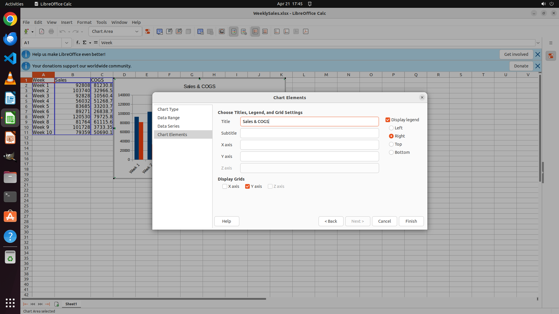
The chart title "Sales & COGS" has been successfully entered in the Title field. I can see:
- The Title field now displays "Sales & COGS"
- The chart preview at the top shows the title displayed above the chart
- The chart configuration is complete with:
- Column chart type (clustered)
- Data series: Sales and COGS
- Categories: Week 1-10
- Title: Sales & COGS
- Legend displayed on the right
#### 情况分析与思考过程
Current progress on the strategy tree:
1. ✓ Select source data range in Sheet1 (completed)
2. → Insert and configure clustered column chart (almost complete)
- ✓ Open Insert menu and select Chart (completed)
- ✓ Select Column chart type and Clustered Column subtype (completed)
- ✓ Set chart title to 'Sales & COGS' (completed)
- Complete chart creation by clicking Finish (current step)
3. Create destination worksheet "Sheet2" (pending)
4. Move chart to Sheet2 (pending)
Now I need to click the "Finish" button to complete the chart creation. This will create the chart in Sheet1. After that, I'll need to create Sheet2 and move the chart there.
The logical next action is to click the "Finish" button to complete the chart creation process.
```
Step 9: RIGHT_CLICK (244, 1045)
```
#### 重要信息
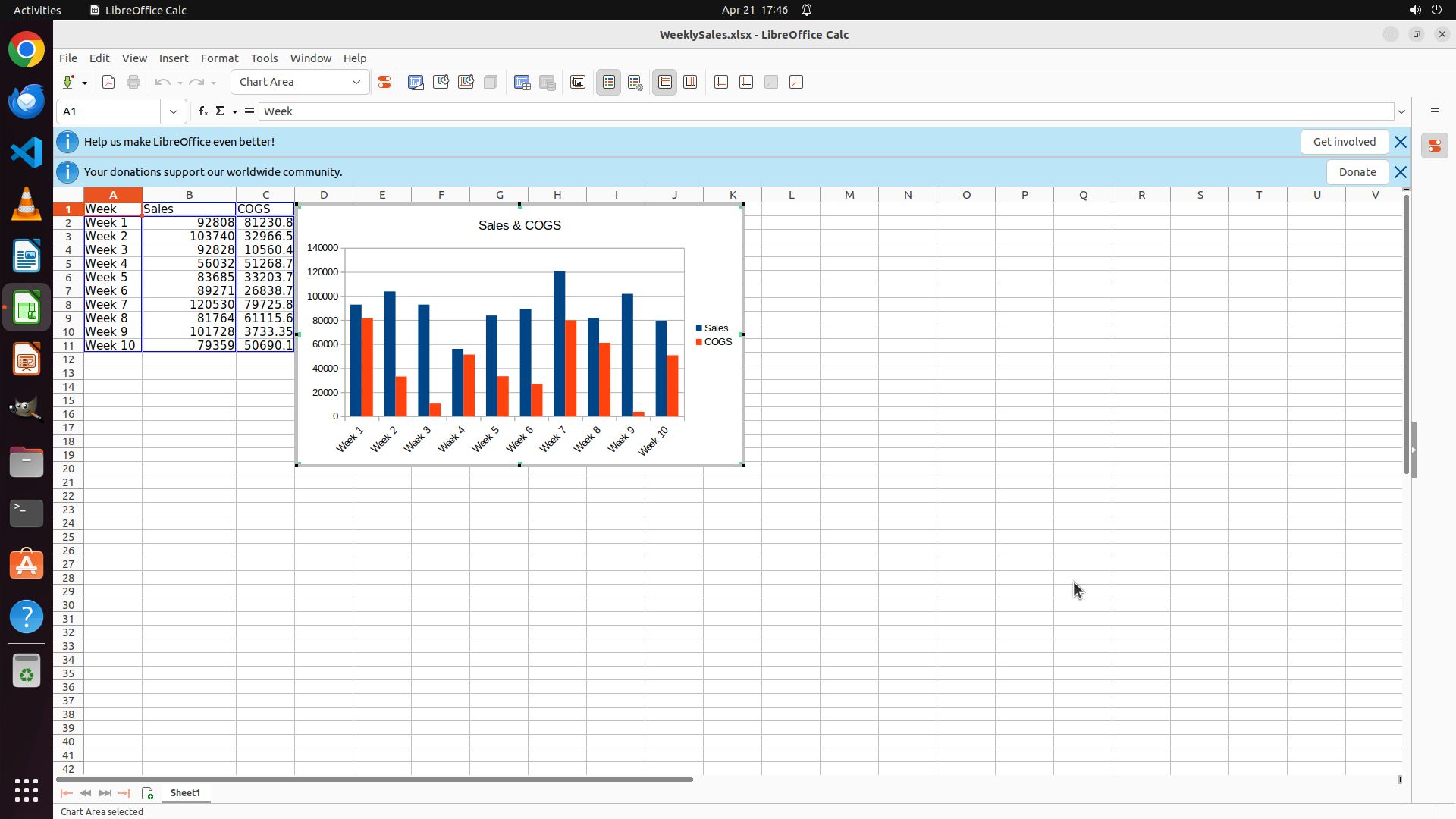
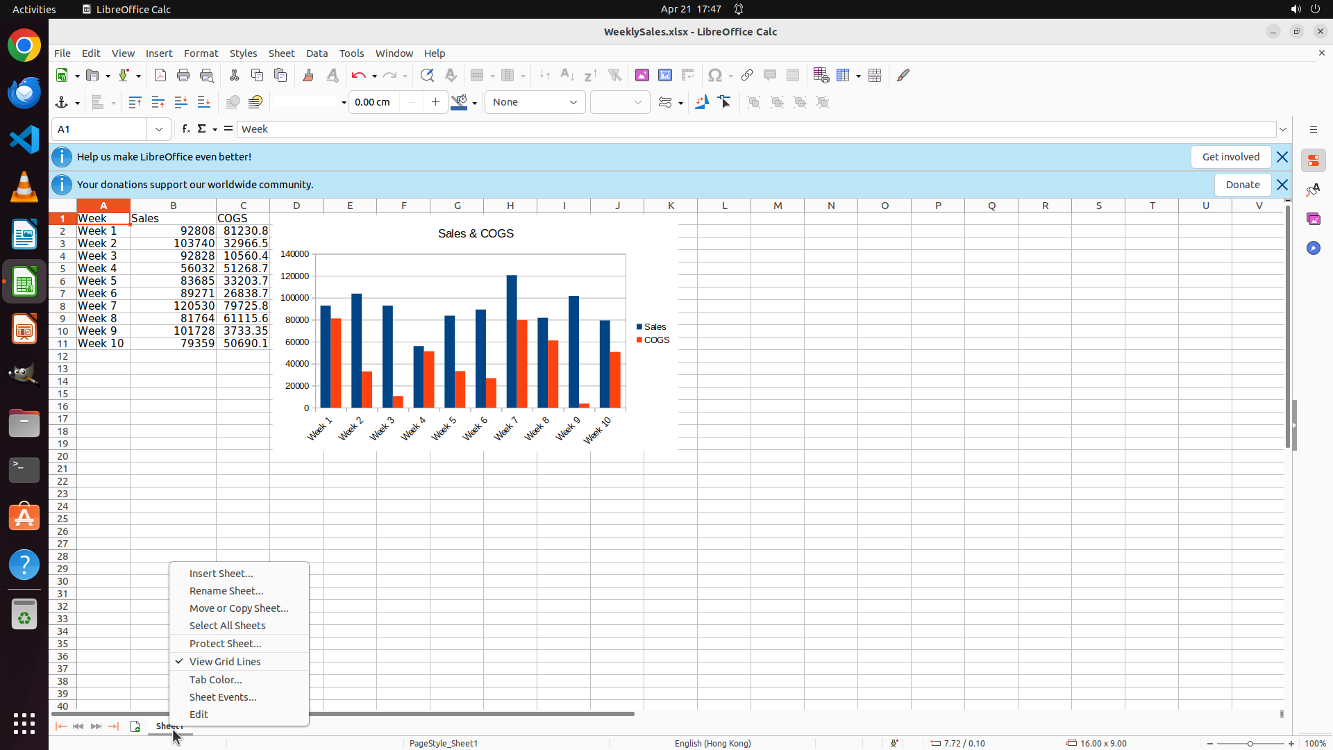
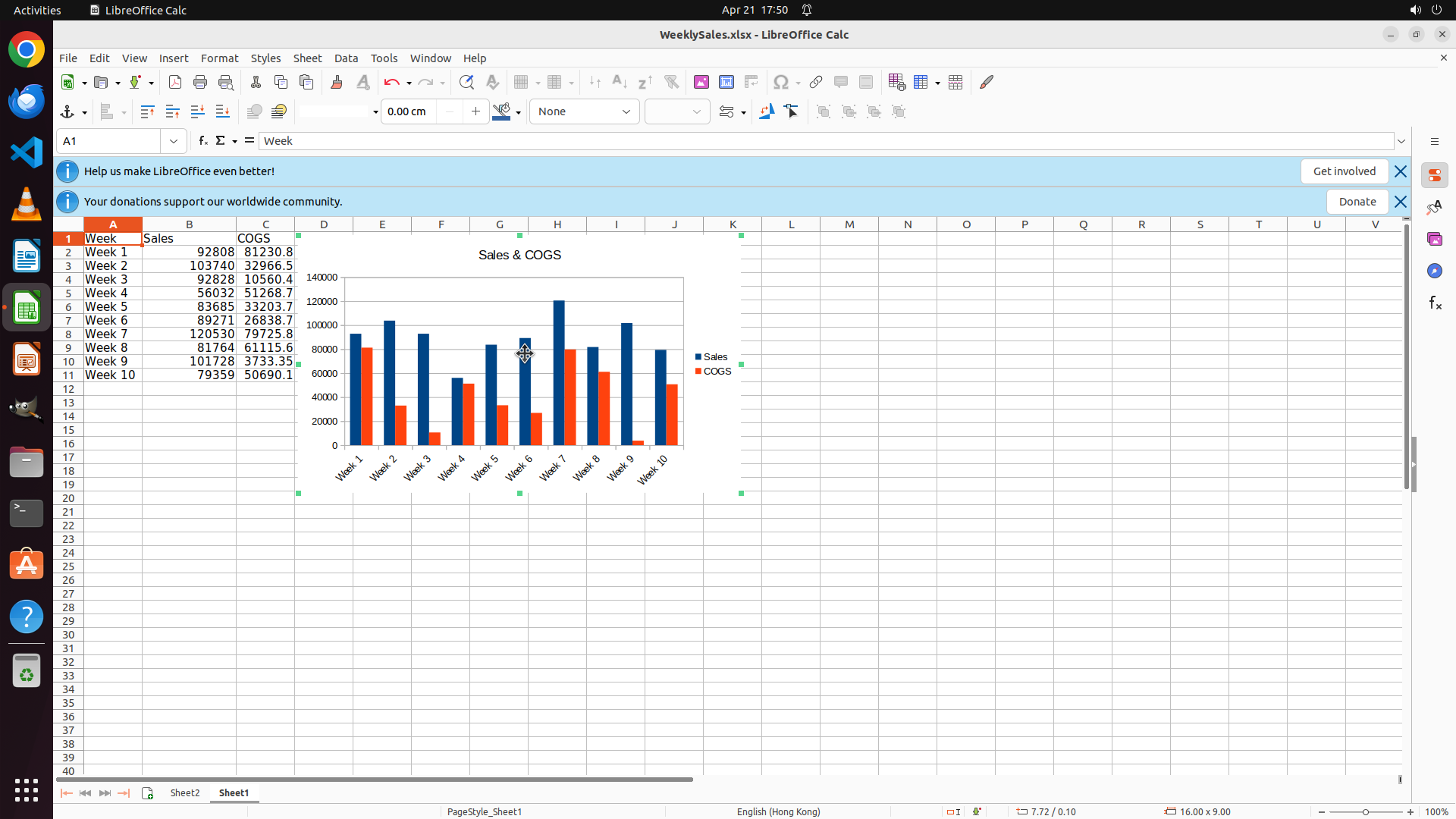
The chart has been successfully created in Sheet1. I can see:
- A clustered column chart with the title "Sales & COGS" displayed at the top
- The chart shows two data series: Sales (blue columns) and COGS (orange/red columns)
- Week 1-10 labels on the X-axis
- A legend on the right showing "Sales" and "COGS"
- The chart is currently selected (selection handles visible)
- The "Sheet1" tab is active at the bottom
- Status bar shows "Chart Area selected"
#### 情况分析与思考过程
Current progress on the strategy tree:
1. ✓ Select source data range in Sheet1 (completed)
2. ✓ Insert and configure clustered column chart (completed)
- ✓ Open Insert menu and select Chart (completed)
- ✓ Select Column chart type and Clustered Column subtype (completed)
- ✓ Set chart title to 'Sales & COGS' (completed)
- ✓ Complete chart creation (completed - chart is now in Sheet1)
3. → Create destination worksheet "Sheet2" (current step)
- 3.1: Right-click on Sheet1 tab and select Insert Sheet (next action)
- 3.2: Enter 'Sheet2' as the sheet name
4. Move chart to Sheet2 (pending)
- 4.1: Cut the chart from Sheet1
- 4.2: Activate Sheet2 and paste the chart
Now I need to create a new sheet named "Sheet2". The logical next action is to right-click on the "Sheet1" tab at the bottom of the screen to open the context menu, which should contain an option to insert a new sheet.
```
Step 10: CLICK (317, 825)
```
#### 重要信息
The right-click on Sheet1 tab successfully opened the context menu. I can see:
- A context menu with various sheet options
- "Insert Sheet..." option is visible at the top of the menu
- The chart is still visible in Sheet1 with the title "Sales & COGS"
- The chart shows clustered columns for Sales (blue) and COGS (orange/red) for Weeks 1-10
#### 情况分析与思考过程
Current progress on the strategy tree:
1. ✓ Select source data range in Sheet1 (completed)
2. ✓ Insert and configure clustered column chart (completed)
- ✓ Open Insert menu and select Chart (completed)
- ✓ Select Column chart type and Clustered Column subtype (completed)
- ✓ Set chart title to 'Sales & COGS' (completed)
- ✓ Complete chart creation (completed - chart is now in Sheet1)
3. → Create destination worksheet "Sheet2" (current step)
- → 3.1: Right-click on Sheet1 tab and select Insert Sheet (context menu is open, need to click "Insert Sheet...")
- 3.2: Enter 'Sheet2' as the sheet name
4. Move chart to Sheet2 (pending)
- 4.1: Cut the chart from Sheet1
- 4.2: Activate Sheet2 and paste the chart
The context menu is now open. I need to click on "Insert Sheet..." to proceed with creating a new sheet. This will open a dialog where I can name the sheet "Sheet2".
```
Step 11: CLICK (1233, 793)
```
#### 重要信息
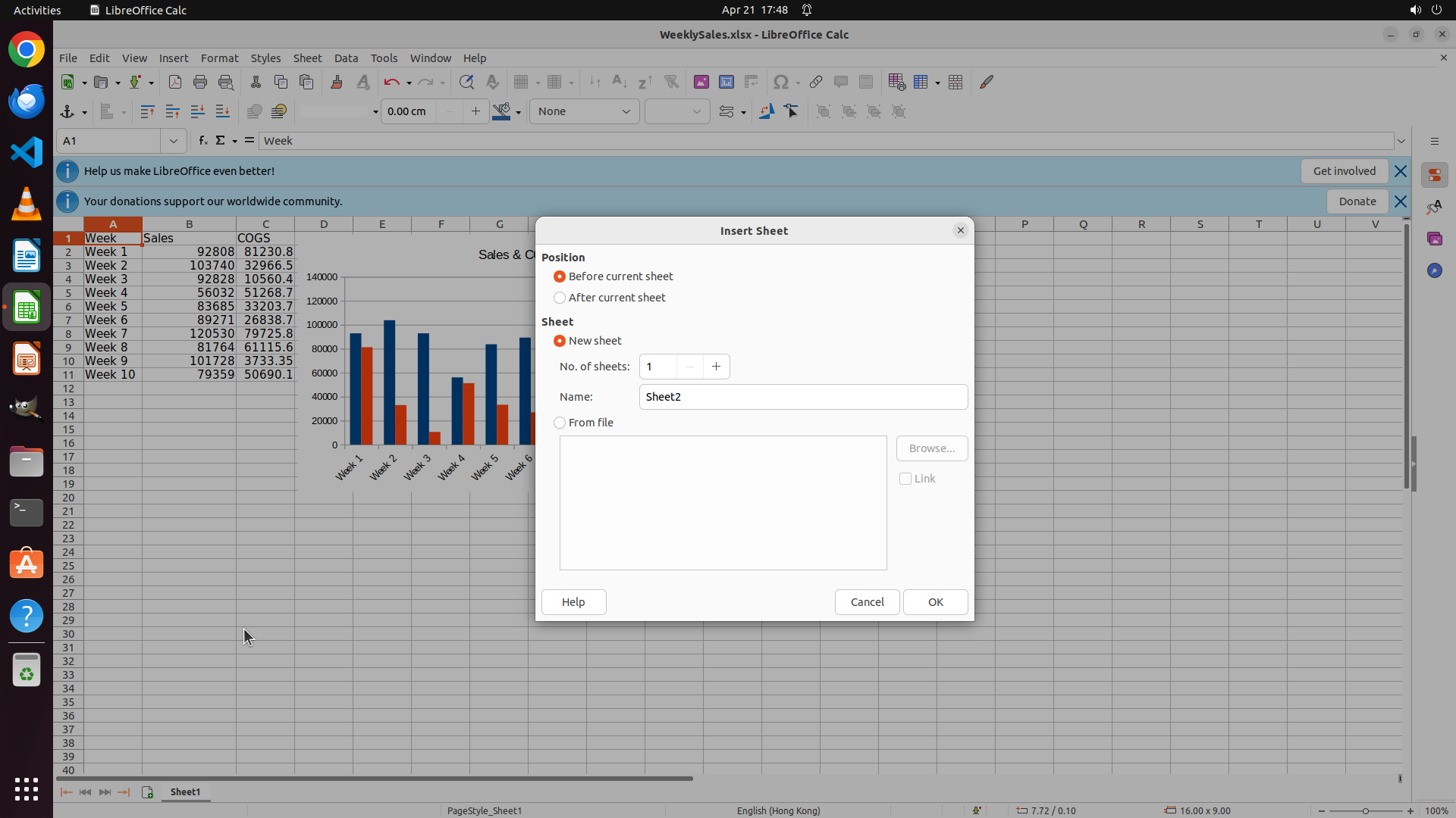
The "Insert Sheet" dialog has opened successfully. I can see:
- The dialog is titled "Insert Sheet"
- "New sheet" radio button is selected
- The Name field already contains "Sheet2" - perfect, this is exactly what we need!
- Position is set to "Before current sheet"
- Number of sheets is set to 1
- Buttons at the bottom: Help, Cancel, OK
#### 情况分析与思考过程
Current progress on the strategy tree:
1. ✓ Select source data range in Sheet1 (completed)
2. ✓ Insert and configure clustered column chart (completed)
- ✓ Open Insert menu and select Chart (completed)
- ✓ Select Column chart type and Clustered Column subtype (completed)
- ✓ Set chart title to 'Sales & COGS' (completed)
- ✓ Complete chart creation (completed - chart is now in Sheet1)
3. → Create destination worksheet "Sheet2" (current step)
- → 3.1: Right-click on Sheet1 tab and select Insert Sheet (completed - dialog is open)
- → 3.2: Enter 'Sheet2' as the sheet name (completed - name is already set to "Sheet2")
- Click OK to create the sheet (next action)
4. Move chart to Sheet2 (pending)
- 4.1: Cut the chart from Sheet1
- 4.2: Activate Sheet2 and paste the chart
The sheet name is already set to "Sheet2" which is exactly what we need. Now I just need to click the "OK" button to create the new sheet. After that, I'll need to cut the chart from Sheet1 and paste it into Sheet2.
```
Step 12: CLICK (305, 1045)
```
#### 重要信息
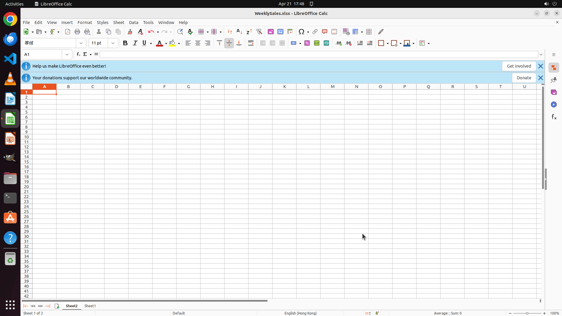
Sheet2 has been successfully created and is now active. I can see:
- The spreadsheet is now showing an empty Sheet2 (blank grid)
- At the bottom, the "Sheet2" tab is active/highlighted
- The status bar shows "Sheet 1 of 2"
- Both "Sheet2" and "Sheet1" tabs are visible at the bottom
- The chart is not visible here because it was created in Sheet1
#### 情况分析与思考过程
Current progress on the strategy tree:
1. ✓ Select source data range in Sheet1 (completed)
2. ✓ Insert and configure clustered column chart (completed)
3. ✓ Create destination worksheet "Sheet2" (completed - Sheet2 is now active)
4. → Move chart to Sheet2 (current step)
- 4.1: Cut the chart from Sheet1 (need to go to Sheet1 first)
- 4.2: Activate Sheet2 and paste the chart
Now I need to go back to Sheet1 to cut the chart. I can see the "Sheet1" tab at the bottom of the screen. I'll click on it to switch to Sheet1 where the chart is located. Once there, I'll select the chart, cut it, then return to Sheet2 and paste it.
The logical next action is to click on the "Sheet1" tab to switch back to Sheet1 where the chart is located.
```
Step 13: CLICK (676, 450)
```
#### 重要信息
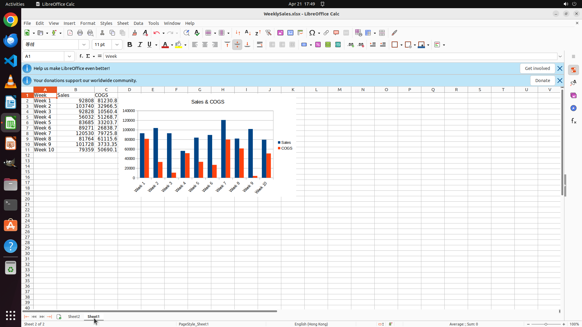
I'm now back in Sheet1 and I can see the clustered column chart with the title "Sales & COGS" displayed. The chart shows:
- Title "Sales & COGS" at the top
- Two data series: Sales (blue columns) and COGS (orange/red columns)
- Week 1-10 labels on the X-axis
- A legend on the right showing "Sales" and "COGS"
- The chart is currently not selected (no selection handles visible)
At the bottom, I can see both "Sheet2" and "Sheet1" tabs, with "Sheet1" currently active.
#### 情况分析与思考过程
Current progress on the strategy tree:
1. ✓ Select source data range in Sheet1 (completed)
2. ✓ Insert and configure clustered column chart (completed)
- All sub-steps completed
3. ✓ Create destination worksheet "Sheet2" (completed)
4. → Move chart to Sheet2 (current step)
- → 4.1: Cut the chart from Sheet1 (need to select chart first, then cut)
- 4.2: Activate Sheet2 and paste the chart
Now I need to:
1. Click on the chart to select it
2. Cut it using Ctrl+X
3. Click on Sheet2 tab to switch to Sheet2
4. Paste the chart using Ctrl+V
The logical next action is to click on the chart to select it. I'll click somewhere in the chart area to select the entire chart object.
```
Step 14: HOTKEY
```
#### 重要信息
The chart is now selected - I can see selection handles (small squares) around the chart border. The chart displays:
- Title "Sales & COGS" at the top
- Two data series: Sales (blue columns) and COGS (orange/red columns)
- Week 1-10 labels on the X-axis
- A legend on the right showing "Sales" and "COGS"
- Selection handles are visible, indicating the chart is selected
At the bottom, I can see both "Sheet2" and "Sheet1" tabs, with "Sheet1" currently active.
#### 情况分析与思考过程
Current progress on the strategy tree:
1. ✓ Select source data range in Sheet1 (completed)
2. ✓ Insert and configure clustered column chart (completed)
3. ✓ Create destination worksheet "Sheet2" (completed)
4. → Move chart to Sheet2 (current step)
- → 4.1: Cut the chart from Sheet1 (chart is selected, now need to cut it)
- 4.2: Activate Sheet2 and paste the chart
The chart is now selected with visible selection handles. The next logical step is to cut the chart using Ctrl+X. After cutting, I'll need to:
1. Click on the Sheet2 tab to switch to Sheet2
2. Paste the chart using Ctrl+V
I'll use the Ctrl+X keyboard shortcut to cut the selected chart.
```
Step 15: CLICK (244, 1045)
```
#### 重要信息
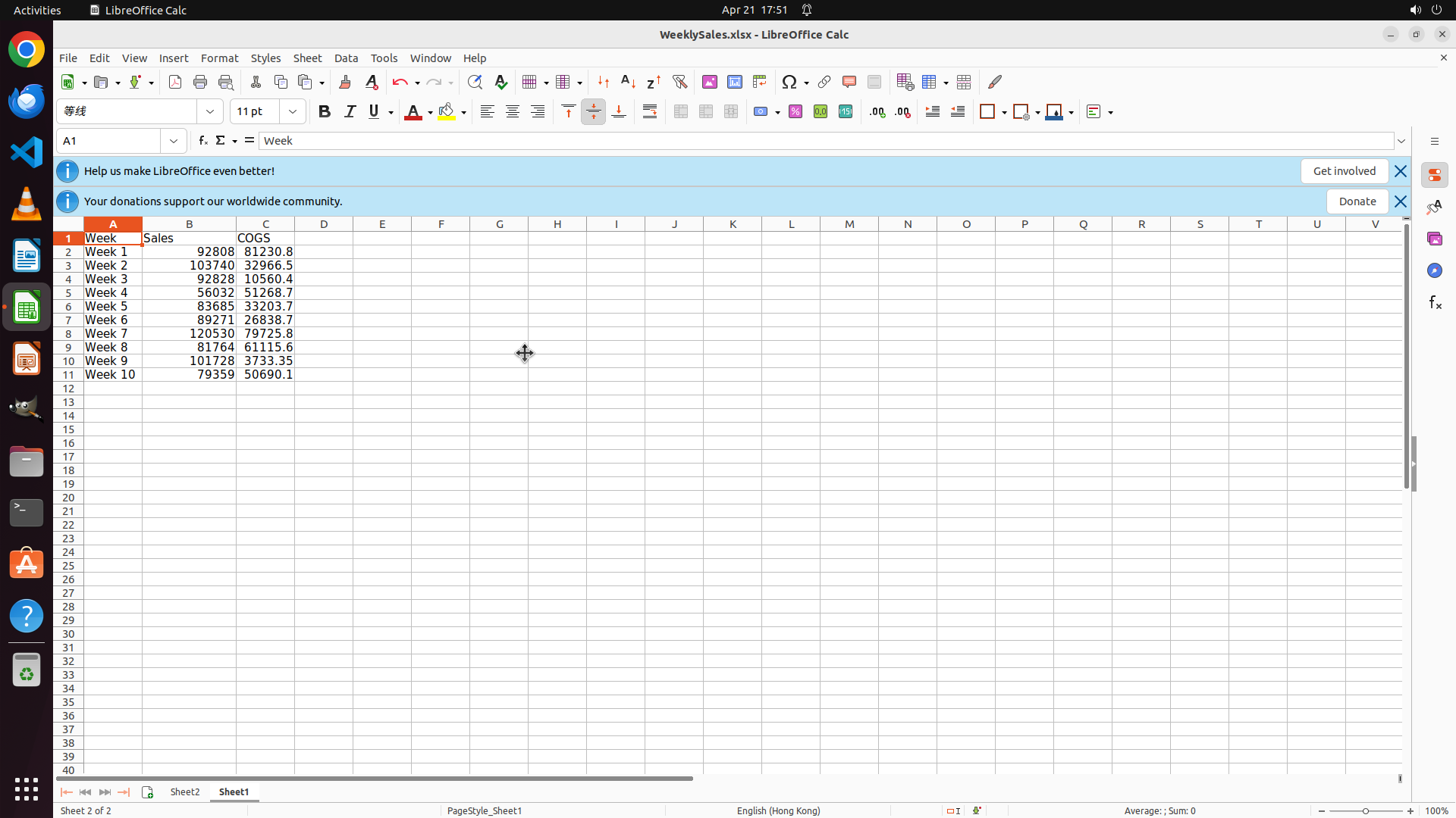
The chart has been successfully cut from Sheet1. I can see:
- Sheet1 is currently active (shown at the bottom)
- The chart is NO LONGER VISIBLE in Sheet1 - only the data table remains
- The data shows Week, Sales, and COGS columns (rows 1-11)
- Both "Sheet2" and "Sheet1" tabs are visible at the bottom of the screen
- The status bar shows "Sheet 1 of 2"
The cut operation (Ctrl+X) was successful as the chart has disappeared from Sheet1.
#### 情况分析与思考过程
Current progress on the strategy tree:
1. ✓ Select source data range in Sheet1 (completed)
2. ✓ Insert and configure clustered column chart (completed)
3. ✓ Create destination worksheet "Sheet2" (completed)
4. → Move chart to Sheet2 (current step)
- ✓ 4.1: Cut the chart from Sheet1 (completed - chart is no longer visible in Sheet1)
- → 4.2: Activate Sheet2 and paste the chart (next step)
Now I need to:
1. Click on the Sheet2 tab to switch to Sheet2
2. Paste the chart using Ctrl+V
After pasting, the chart should appear in Sheet2, completing the task. The chart should retain all its properties including:
- Title "Sales & COGS"
- Clustered column chart type
- Sales and COGS data series
- Week 1-10 labels
The logical next action is to click on the "Sheet2" tab to activate Sheet2, then paste the chart there.
```
I'll click on the Sheet2 tab and then paste the chart.
Step 15: HOTKEY
```
#### 重要信息
The chart has been successfully cut from Sheet1. I can see:
- Sheet1 is currently active (shown at the bottom)
- The chart is NO LONGER VISIBLE in Sheet1 - only the data table remains
- The data shows Week, Sales, and COGS columns (rows 1-11)
- Both "Sheet2" and "Sheet1" tabs are visible at the bottom of the screen
- The status bar shows "Sheet 1 of 2"
The cut operation (Ctrl+X) was successful as the chart has disappeared from Sheet1.
#### 情况分析与思考过程
Current progress on the strategy tree:
1. ✓ Select source data range in Sheet1 (completed)
2. ✓ Insert and configure clustered column chart (completed)
3. ✓ Create destination worksheet "Sheet2" (completed)
4. → Move chart to Sheet2 (current step)
- ✓ 4.1: Cut the chart from Sheet1 (completed - chart is no longer visible in Sheet1)
- → 4.2: Activate Sheet2 and paste the chart (next step)
Now I need to:
1. Click on the Sheet2 tab to switch to Sheet2
2. Paste the chart using Ctrl+V
After pasting, the chart should appear in Sheet2, completing the task. The chart should retain all its properties including:
- Title "Sales & COGS"
- Clustered column chart type
- Sales and COGS data series
- Week 1-10 labels
The logical next action is to click on the "Sheet2" tab to activate Sheet2, then paste the chart there.
```
I'll click on the Sheet2 tab and then paste the chart.
Step 16: HOTKEY
```
#### 重要信息
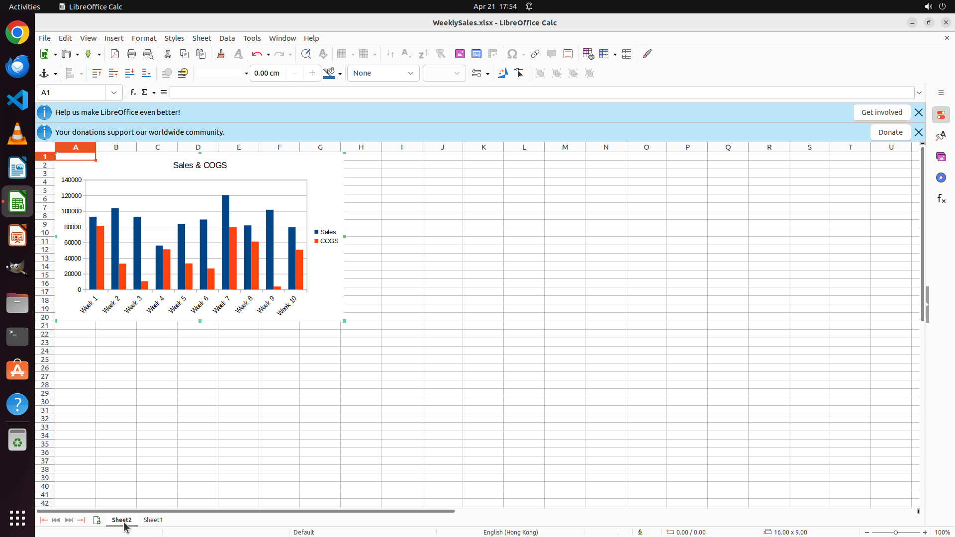
The chart has been successfully pasted into Sheet2! I can see:
- Sheet2 is currently active (the "Sheet2" tab is highlighted at the bottom)
- The clustered column chart is now visible in Sheet2 with the title "Sales & COGS" displayed at the top
- The chart shows Week 1-10 labels on the X-axis
- Two data series are displayed: Sales (blue columns) and COGS (orange/red columns)
- The legend on the right shows both "Sales" and "COGS" labels
- The chart is properly formatted as a clustered column chart
All task requirements have been met:
✓ Clustered column chart created
✓ Shows Sales and COGS data for each week
✓ Located in a new sheet named "Sheet2"
✓ Chart title set as "Sales & COGS"
#### 情况分析与思考过程
Current progress on the strategy tree:
1. ✓ Select source data range in Sheet1 (completed)
2. ✓ Insert and configure clustered column chart (completed)
- All sub-steps completed
3. ✓ Create destination worksheet "Sheet2" (completed)
4. ✓ Move chart to Sheet2 (completed)
- ✓ 4.1: Cut the chart from Sheet1 (completed)
- ✓ 4.2: Activate Sheet2 and paste the chart (completed - chart is now visible in Sheet2)
The task has been successfully completed! All the key visual evidence requirements are satisfied:
- The 'Sheet2' tab is visible and active at the bottom
- A clustered column chart object is present in Sheet2
- The chart title displays 'Sales & COGS'
- The chart shows clustered columns with Week 1-10 labels and two data series (Sales and COGS)
- The chart legend shows both 'Sales' and 'COGS' series labels
I should now update the strategy tree to mark the task as complete and save the file to ensure the changes are preserved.
```